Alternative Data for Energy Markets: Implementation and Empirical Validation

Abstract

This article documents three independent investigations into alternative data sources for energy market signals: satellite imagery for oil storage estimation, maritime vessel tracking for commodity flows, and pipeline capacity modeling for natural gas basis volatility. Each study followed a hypothesis-driven approach, applying quantitative methods to publicly available or low-cost data sources. The findings illustrate both the potential and the significant limitations of alternative data in generating actionable trading signals.

---

Introduction

Alternative data has attracted considerable attention from quantitative investors seeking informational edges in commodity markets. The premise is intuitive: physical commodity flows leave observable traces (ships move, tanks fill, pipelines operate) and these traces may contain information not yet reflected in prices.

I investigated three distinct alternative data sources across the energy complex:

1. Satellite Imagery: Estimating crude oil inventory at Cushing, Oklahoma using commercial satellite imagery and computer vision
2. AIS Vessel Tracking: Analyzing 1.13 billion maritime vessel positions to predict oil prices and energy equities
3. Pipeline Capacity Modeling: Building a physical model of Permian Basin natural gas takeaway constraints to identify volatility mispricings

Each investigation followed a consistent methodology: define a falsifiable hypothesis, acquire relevant data, implement a quantitative framework, and rigorously validate against out-of-sample data or known ground truth. The results varied considerably: some hypotheses failed outright, others showed promise in narrow contexts, and several revealed fundamental limitations in the alternative data thesis itself.

---

Study 1: Satellite-Based Oil Storage Estimation

Hypothesis

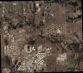
Floating-roof oil storage tanks at Cushing, Oklahoma, the delivery point for WTI futures, exhibit observable shadow patterns that correlate with fill levels. By detecting tanks and measuring shadow characteristics via satellite imagery, one could estimate aggregate inventory levels before official EIA releases.

Data Sources

Source	Resolution	Cost	Purpose
Sentinel-2 (ESA)	10m/pixel	Free	Initial feasibility
SPOT 6/7 (Airbus)	1.5m/pixel	~$70/image	Volume estimation
Kaggle Oil Tanks Dataset	Various	Free	Model training
EIA Weekly Petroleum Report	—	Free	Ground truth

SPOT imagery was purchased through my LLC, as the service I used (UP42) does not sell to individuals.

Methodology

I trained a YOLOv8 object detection model on approximately 8,000 annotated tank images, achieving 96.2% mAP@50 on held-out test data. The model was applied to satellite imagery of Cushing using tiled inference with non-maximum suppression to handle large image dimensions.

For volume estimation, the academic literature suggests measuring the ratio of interior shadow (on the floating roof) to exterior shadow (cast by tank walls). I implemented this approach using HSV/LAB color space transformations to enhance shadow regions.

Results

Tank Detection: The detection model performed well at 1.5m resolution, identifying 75-158 tanks per image depending on confidence thresholds. At 10m resolution (Sentinel-2), detection degraded significantly; tanks appeared as only 5-8 pixels, insufficient for reliable identification.

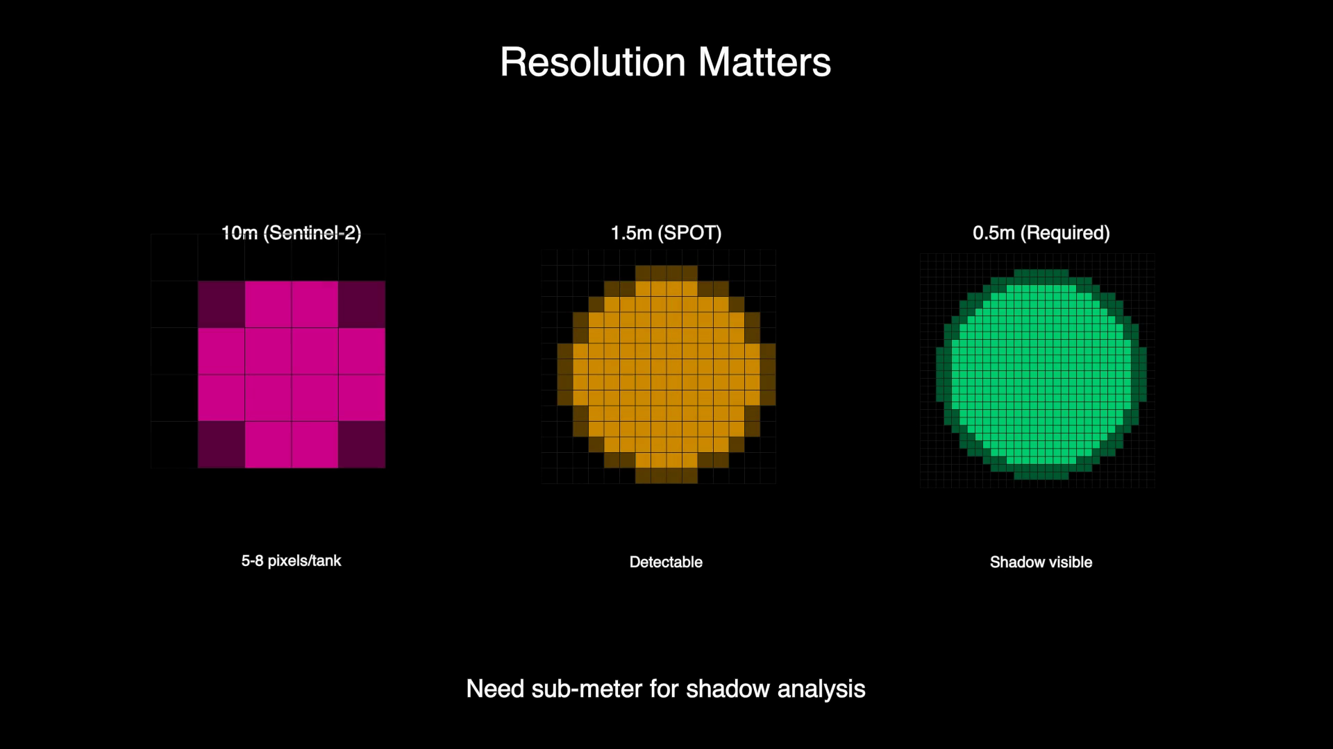
Volume Estimation: The shadow-based volume estimation approach failed. At 1.5m resolution, exterior shadows were not reliably distinguishable from tank perimeters and ground features. The shadow enhancement formula produced occupancy estimates of 0% for all tanks, a clear indicator of methodological failure.

I pivoted to a simpler brightness-based heuristic (brighter interior = fuller tank), which produced varying occupancy estimates. However, validation against EIA data revealed fundamental problems:

Metric	EIA Ground Truth	Satellite Estimate
November 2023	23.1M barrels	14.8M barrels
November 2024	24.2M barrels	18.0M barrels
Direction	+4.8%	+22%

While directional agreement was achieved (both showed inventory increases), the magnitude discrepancy and the fact that I detected only ~22% of Cushing’s 350+ tanks renders the absolute estimates unreliable.

Conclusions

The hypothesis that shadow-based volume estimation could work at 1.5m resolution was falsified. The minimum viable resolution for true shadow analysis appears to be 0.5m or better, which increases imagery costs by 3-5x. The brightness-based fallback method lacks physical grounding and showed inconsistent calibration.

For satellite-based oil inventory to be viable at Cushing specifically, one would need: (a) sub-meter resolution imagery, (b) complete coverage of all storage facilities, and (c) calibration data spanning multiple inventory cycles. The $140 spent on imagery successfully answered the feasibility question: negatively.

---

Study 2: Maritime AIS Data for Energy Market Signals

Hypothesis

Automatic Identification System (AIS) vessel tracking data contains information about physical commodity flows that may predict energy prices. Specifically, I hypothesized that tanker counts in key maritime zones (Gulf of Mexico, Houston Ship Channel, Sabine Pass LNG terminal) would correlate with oil prices, natural gas prices, and energy equities.

Data Sources

Source	Coverage	Records	Cost
Marine Cadastre (NOAA)	US coastal waters, 2018-2024	6+ billion positions	Free
Polygon.io	US equities and ETFs	4 years daily	$29/month

Methodology

I processed 1.13 billion AIS positions for 2018-2024, filtering for tanker and cargo vessel types within defined geographic zones. Daily vessel counts were computed and tested for correlation with various financial instruments including USO (oil ETF), UNG (natural gas ETF), XLE (energy sector ETF), and individual tanker company stocks.

Signals passing initial correlation screening (r > 0.15, p < 0.05) were subjected to out-of-sample backtesting using a train/test split methodology.

Results

Failed Hypotheses:

The majority of intuitive hypotheses failed validation:

Hypothesis	Correlation	Backtest Result	Failure Mode
Gulf tankers → Oil prices	r = 0.29	-20% return	Sign flips monthly
Sabine Pass LNG vessels → UNG	r = 0.14	Not tested	Too few vessels (0.9/day)
LA/Long Beach cargo → ZIM stock	r = 0.46	-17% return	Spurious (common macro driver)
Week-over-week changes	r = 0.02	—	No signal
Deseasonalized counts	r < 0.06	—	No signal

The Gulf tanker correlation of r = 0.29 appeared promising in aggregate but decomposed poorly: monthly correlations ranged from r = -0.74 (June) to r = +0.67 (September), indicating an unstable relationship unsuitable for systematic trading.

Partial Success: Extreme Events

One approach showed modest promise, trading only on extreme readings (>1.5 standard deviations from mean):

Metric	Value
Total trades	15
Win rate	53%
Sharpe ratio	2.13

However, the low trade count (15 per year) provides insufficient statistical confidence, and out-of-sample testing showed degradation (Sharpe 0.91).

Feature Engineering Attempts:

I computed additional features including vessel draft (loaded vs. empty), size classes, flag states, and speed. Some features showed high in-sample correlations:

Feature	In-Sample Correlation	Out-of-Sample Sharpe
draft_empty	r = 0.36	0.00 (1 trade)
size_small	r = 0.35	2.89 (6 trades)
flag_us	r = 0.26	1.91 (17 trades)

The strongest in-sample signal (draft_empty) failed completely out-of-sample, producing only one trade that lost money. This exemplifies the overfitting risk in alternative data research.

Pivot to Tanker Equities:

The most notable finding was that AIS data showed stronger relationships with tanker company stocks (FRO, STNG, TNK) than with oil prices directly. This makes economic sense: tanker company revenues are directly tied to vessel utilization, while oil prices respond to a complex mix of OPEC decisions, geopolitics, and macroeconomic factors.

However, high correlations (r = 0.90+) between AIS features and tanker stocks likely reflect common trending behavior rather than causal predictive power.

Conclusions

The hypothesis that raw AIS vessel counts predict oil prices was falsified. The relationship is unstable across time, reverses sign frequently, and does not survive rigorous backtesting.

Alternative formulations (extreme events, specific vessel characteristics) showed marginal promise but with trade counts too low for statistical confidence. The finding that AIS data relates more strongly to tanker equities than commodity prices suggests potential, but requires longer history and careful detrending to distinguish causation from coincident trending.

The core lesson: correlation does not imply causation, and neither implies a tradeable signal.

---

Study 3: Permian Basin Pipeline Capacity Modeling

Hypothesis

Natural gas production in the Permian Basin is “forced” (associated gas from oil wells), making pipeline takeaway capacity the binding constraint. When production exceeds takeaway capacity, Waha Hub prices collapse nonlinearly. This convexity may be underpriced by options markets, creating opportunity for a conditional overlay that times exposure to long-volatility positions.

Approach

Rather than beginning with price data (which risks overfitting), I constructed a physical model of pipeline capacity from primary sources:

Pipelines Modeled:

Pipeline	Nameplate Capacity	Delivery Zone
Gulf Coast Express (GCX)	2.00 Bcf/d	Agua Dulce
Permian Highway (PHP)	2.10 Bcf/d	Katy Hub
Whistler	2.00 Bcf/d	Agua Dulce

Data Sources:

• Kinder Morgan Electronic Bulletin Board (maintenance notices)
• Bloomberg Terminal (Waha Hub spot prices, NGTXOASI Index)

Methodology

I parsed actual maintenance notices from pipeline operator filings, extracting capacity reduction events with start dates, end dates (if known), and affected volumes. A key modeling decision was treating open-ended events (unknown end date) as first-class objects rather than imputing durations.

From these primitives, I computed daily system state including effective capacity, event overlap counts, and uncertainty flags. Days were classified into stress regimes (Normal, Stressed, Disrupted) based on capacity reduction thresholds.

A “Convexity Score” was defined to quantify option-relevant stress:

• +1 if capacity loss >= 8%
• +1 if event overlap >= 2
• +1 if open-ended (duration uncertain)
• +1 if stress duration >= 2 days

The score was frozen before examining price data.

Volatility Alignment Analysis

I then asked: when physical stress is high, does market volatility respond appropriately?

Using Waha Hub spot prices, I computed realized volatility in windows before, during, and after stress events. The alignment diagnosis categorized market response as:

• Aligned: Volatility matched physical stress
• VolLagged: Volatility increased late
• VolUndershot: Volatility increase was insufficient
• VolRevertedEarly: Volatility normalized before stress resolved

Results

Stress Event Identification:

Window	Duration	Regime	Convexity Score
Sep 17-18, 2025	2 days	Stressed	4/4
Oct 21-23, 2025	3 days	Disrupted	4/4

Volatility Behavior:

For the September window, volatility correctly spiked 3x during stress but reverted to baseline levels while an open-ended outage remained unresolved. This pattern (VolRevertedEarly) suggests potential underpricing of persistence risk.

Conditional Overlay Test:

I tested a simple rule: hold long-volatility exposure only when ConvexityScore >= 3 AND diagnosis indicates market underpricing.

Metric	Always-On	Overlay-Conditioned
Exposure ratio	100%	1.0%
Exposure days	503	5
Mean P&L (exposed)	+$0.34/day	+$0.56/day
Std Dev (exposed)	$0.97	$0.50
Conditional Sharpe	+5.62	+17.85
Max drawdown	$10.14	$0.00

Limitations

Several factors limit confidence in these results:

1. Sample size: Only 5 exposure days from 2 stress windows is insufficient for statistical significance
2. P&L proxy: I used absolute price changes minus median as a proxy for long-volatility P&L, which is a simplification
3. Selection bias: My hand-curated maintenance notices contain only severe events; benign events were not tested
4. Single pipeline system: Only GCX was modeled; PHP and Whistler notices were not incorporated
5. No options data: Actual implied volatility data was not available to verify the “underpricing” hypothesis

Conclusions

The physical model of pipeline capacity constraints successfully identifies periods of elevated stress. The observation that volatility reverts before open-ended outages resolve is suggestive of potential mispricing.

However, the strategy cannot be validated with the available data. The improvement in conditional Sharpe may reflect variance reduction (a robust finding) or may be an artifact of favorable sample selection (5 days from a limited dataset). Distinguishing between these explanations requires substantially more data across multiple stress cycles.

The approach demonstrates how alternative data research should proceed (mechanism first, falsifiable hypotheses, price data introduced only after the physical model is sound) but the findings themselves remain preliminary.

---

Cross-Study Observations

What Worked

1. Clear hypothesis definition: Each study began with a specific, falsifiable claim
2. Appropriate ground truth: EIA data for oil storage, out-of-sample backtests for AIS, pipeline filings for capacity
3. Honest failure recognition: Shadow-based volume estimation was abandoned when it failed; most AIS hypotheses were rejected
4. Physical reasoning: The pipeline capacity study’s mechanism-first approach avoided data mining

What Did Not Work

1. Resolution limitations: 1.5m satellite imagery was insufficient for shadow analysis; 10m was insufficient for tank detection
2. Correlation-causation confusion: High AIS correlations decomposed under scrutiny
3. Sample size constraints: The pipeline study’s 5 exposure days cannot support confident conclusions
4. Overfitting risk: The strongest in-sample AIS signal (draft_empty) failed completely out-of-sample

The Alternative Data Thesis

These studies suggest that alternative data for commodity markets faces structural challenges:

1. Signal-to-noise ratio: Physical flows are noisy proxies for the economic variables that actually drive prices
2. Latency: By the time satellite imagery is acquired and processed, the information may already be reflected in prices
3. Coverage: Partial observation (22% of Cushing tanks, US-only AIS) limits reliability
4. Stationarity: Relationships that hold in one period may not persist

None of this implies alternative data is without value. Rather, it suggests that naive applications (correlate alternative data with prices, backtest, deploy) are unlikely to succeed. Value may exist in narrower contexts: using AIS to predict tanker company earnings rather than oil prices, or using pipeline capacity data as one input among many in a fundamental model.

---

Technical Implementation

Infrastructure

Component	Specification
Compute	Vultr bare metal (16 CPU, 128GB RAM, 1.8TB NVMe)
Database	PostgreSQL 16 with PostGIS
ML Framework	PyTorch, Ultralytics YOLOv8
Languages	Python (data processing), Rust (pipeline model)

Data Processing Performance

Task	Volume	Time
AIS loading (1 year)	1.13B rows	40 minutes
AIS loading (7 years)	~6B rows	~12 hours
Satellite tile inference	4296x3796 px	~30 seconds
Feature computation	2557 days	~10 hours

Cost Summary

Item	Cost
SPOT satellite imagery (2 images)	$140
Polygon.io subscription	$29/month
Vultr compute (as needed)	~$50 total
Databento credits	$125 (free tier)
Total	~$350

---

Conclusion

Three investigations into alternative data for energy markets yielded mixed results. Satellite-based oil storage estimation requires higher resolution than commercially practical. Maritime vessel tracking shows weak and unstable relationships with commodity prices, though potentially stronger relationships with shipping equities warrant further study. Pipeline capacity modeling demonstrates a sound methodological approach but lacks sufficient data for validation.

The broader lesson is methodological: alternative data research requires rigorous hypothesis testing, appropriate ground truth, out-of-sample validation, and honest acknowledgment of limitations. The temptation to find patterns in novel data sources is strong; the discipline to reject those patterns when they fail validation is essential.

---

The analyses described in this article were conducted as independent research projects. No trading decisions were made based on these findings. All data sources are publicly available or commercially accessible.